Analytic Functions Overview - AVG,

Introduced in Oracle 8i, analytic functions, also known as windowing functions, allowed developers to perform tasks in SQL that were previously confined to procedural languages.

• Introduction

• Analytic Function Syntax

o query_partition_clause

o order_by_clause

o windowing_clause

• Using Analytic Functions

Related articles.

• RANK, DENSE_RANK, FIRST and LAST Analytic Functions

• FIRST_VALUE and LAST_VALUE Analytic Functions

• LAG and LEAD Analytic Functions

• LISTAGG Analystic Function in 11g Release 2

• Top-N Queries

Introduction:-

Probably the easiest way to understand analytic functions is to start by looking at aggregate functions. An aggregate function, as the name suggests, aggregates data from several rows into a single result row. For example, we might use the AVG aggregate function to give us an average of all the employee salaries in the EMP table.

SELECT AVG(sal)
FROM emp;

AVG(SAL)
----------
2073.21429

The GROUP BY clause allows us to apply aggregate functions to subsets of rows. For example, we might want to display the average salary for each department.

SELECT deptno, AVG(sal)
FROM emp
GROUP BY deptno
ORDER BY deptno;

DEPTNO AVG(SAL)
---------- ----------
10 2916.66667
20 2175
30 1566.66667

In both cases, the aggregate function reduces the number of rows returned by the query.

Analytic functions also operate on subsets of rows, similar to aggregate functions in GROUP BY queries, but they do not reduce the number of rows returned by the query. For example, the following query reports the salary for each employee, along with the average salary of the employees within the department.

SELECT empno, deptno, sal,
AVG(sal) OVER (PARTITION BY deptno) AS avg_dept_sal
FROM emp;

EMPNO DEPTNO SAL AVG_DEPT_SAL
---------- ---------- ---------- ------------
7782 10 2450 2916.66667
7839 10 5000 2916.66667
7934 10 1300 2916.66667
7566 20 2975 2175
7902 20 3000 2175
7876 20 1100 2175
7369 20 800 2175
7788 20 3000 2175
7521 30 1250 1566.66667
7844 30 1500 1566.66667
7499 30 1600 1566.66667
7900 30 950 1566.66667
7698 30 2850 1566.66667
7654 30 1250 1566.66667

This time AVG is an analytic function, operating on the group of rows defined by the contents of the OVER clause. This group of rows is known as a window, which is why analytic functions are sometimes referred to as window[ing] functions. Notice how the AVG function is still reporting the departmental average, like it did in the GROUP BY query, but the result is present in each row, rather than reducing the total number of rows returned. This is because analytic functions are performed on a result set after all join, WHERE, GROUP BY and HAVING clauses are complete, but before the final ORDER BY operation is performed.

Analytic Function Syntax:

There are some variations in the syntax of the individual analytic functions, but the basic syntax for an analytic function is as follows:

    analytic_function([ arguments ]) OVER (analytic_clause)

The analytic_clause breaks down into the following optional elements.
     [ query_partition_clause ] [ order_by_clause [ windowing_clause ] ]

The sub-elements of the analytic_clause each have their own syntax diagrams, shown here. Rather than repeat the syntax diagrams, the following sections describe what each section of the analytic_clause is used for.

query_partition_clause:

The query_partition_clause divides the result set into partitions, or groups, of data. The operation of the analytic function is restricted to the boundary imposed by these partitions, similar to the way a GROUP BY clause affects the action of an aggregate function. If the query_partition_clause is omitted, the whole result set is treated as a single partition. The following query uses an empty OVER clause, so the average presented is based on all the rows of the result set.

SELECT empno, deptno, sal,
AVG(sal) OVER () AS avg_sal
FROM emp;

EMPNO DEPTNO SAL AVG_SAL
---------- ---------- ---------- ----------
7369 20 800 2073.21429
7499 30 1600 2073.21429
7521 30 1250 2073.21429
7566 20 2975 2073.21429
7654 30 1250 2073.21429
7698 30 2850 2073.21429
7782 10 2450 2073.21429
7788 20 3000 2073.21429
7839 10 5000 2073.21429
7844 30 1500 2073.21429
7876 20 1100 2073.21429
7900 30 950 2073.21429
7902 20 3000 2073.21429
7934 10 1300 2073.21429

SQL>

If we change the OVER clause to include a query_partition_clause based on the department, the averages presented are specifically for the department the employee belongs too.

SELECT empno, deptno, sal,
AVG(sal) OVER (PARTITION BY deptno) AS avg_dept_sal
FROM emp;

EMPNO DEPTNO SAL AVG_DEPT_SAL
---------- ---------- ---------- ------------
7782 10 2450 2916.66667
7839 10 5000 2916.66667
7934 10 1300 2916.66667
7566 20 2975 2175
7902 20 3000 2175
7876 20 1100 2175
7369 20 800 2175
7788 20 3000 2175
7521 30 1250 1566.66667
7844 30 1500 1566.66667
7499 30 1600 1566.66667
7900 30 950 1566.66667
7698 30 2850 1566.66667
7654 30 1250 1566.66667SQL>

order_by_clause:

The order_by_clause is used to order rows, or siblings, within a partition. So if an analytic function is sensitive to the order of the siblings in a partition you should include an order_by_clause. The following query uses the FIRST_VALUE function to return the first salary reported in each department. Notice we have partitioned the result set by the department, but there is no order_by_clause.

SELECT empno, deptno, sal, 

FIRST_VALUE(sal IGNORE NULLS) OVER (PARTITION BY deptno) AS first_sal_in_dept

FROM emp;

EMPNO DEPTNO SAL FIRST_SAL_IN_DEPT
---------- ---------- ---------- -----------------
7782 10 2450 2450
7839 10 5000 2450
7934 10 1300 2450
7566 20 2975 2975
7902 20 3000 2975
7876 20 1100 2975
7369 20  800 2975
7788 20 3000 2975
7521 30 1250 1250
7844 30 1500 1250
7499 30 1600 1250
7900 30 950 1250
7698 30 2850 1250
7654 30 1250 1250

SQL>

Now compare the values of the FIRST_SAL_IN_DEPT column when we include an order_by_clause to order the siblings by ascending salary.

SELECT empno, deptno, sal, 
FIRST_VALUE(sal IGNORE NULLS) OVER (PARTITION BY deptno ORDER BY sal ASC NULLS LAST) AS first_val_in_dept
FROM emp;

EMPNO DEPTNO SAL FIRST_VAL_IN_DEPT
---------- ---------- ---------- -----------------
7934 10 1300 1300
7782 10 2450 1300
7839 10 5000 1300
7369 20 800 800
7876 20 1100 800
7566 20 2975 800
7788 20 3000 800
7902 20 3000 800
7900 30 950 950
7654 30 1250 950
7521 30 1250 950
7844 30 1500 950
7499 30 1600 950
7698 30 2850 950

SQL>

In this case the "ASC NULLS LAST" keywords are unnecessary as ASC is the default for an order_by_clause and NULLS LAST is the default for ASC orders. When ordering by DESC, the default is NULLS FIRST.

It is important to understand how the order_by_clause affects display order. The order_by_clause is guaranteed to affect the order of the rows as they are processed by the analytic function, but it may not always affect the display order. As a result, you must always use a conventional ORDER BY clause in the query if display order is important. Do not rely on any implicit ordering done by the analytic function. Remember, the conventional ORDER BY clause is performed after the analytic processing, so it will always take precedence.

windowing_clause:

We have seen previously the query_partition_clause controls the window, or group of rows, the analytic operates on. The windowing_clause gives some analytic functions a further degree of control over this window within the current partition. The windowing_clause is an extension of the order_by_clause and as such, it can only be used if an order_by_clause is present. 

The windowing_clause has two basic forms:-

RANGE BETWEEN start_point AND end_point
ROWS BETWEEN start_point AND end_point

Possible values for "start_point" and "end_point" are:
• UNBOUNDED PRECEDING: The window starts at the first row of the partition. Only available for start points.
• UNBOUNDED FOLLOWING: The window ends at the last row of the partition. Only available for end points.
• CURRENT ROW :- The window starts or ends at the current row. Can be used as start or end point.
• value_expr PRECEDING :- A physical or logical offset before the current row using a constant or expression that evaluates to a positive numerical value. When used with RANGE, it can also be an interval literal if the order_by_clause uses a DATE column.
• value_expr FOLLOWING :- As above, but an offset after the current row.

The documentation states the start point must always be before the end point, but this is not true, as demonstrated by this rather silly, but valid, query.

SELECT empno, deptno, sal, 
AVG(sal) OVER (PARTITION BY deptno ORDER BY sal ROWS BETWEEN 0 PRECEDING AND 0 PRECEDING) AS avg_of_current_sal
FROM emp;

EMPNO DEPTNO SAL AVG_OF_CURRENT_SAL
---------- ---------- ---------- ------------------
7934 10 1300 1300
7782 10 2450 2450
7839 10 5000 5000
7369 20 800 800
7876 20 1100 1100
7566 20 2975 2975
7788 20 3000 3000
7902 20 3000 3000
7900 30 950 950
7654 30 1250 1250
7521 30 1250 1250
7844 30 1500 1500
7499 30 1600 1600
7698 30 2850 2850

SQL>

In fact, the start point must be before or equal to the end point.

For analytic functions that support the windowing_clause, the default action is "RANGE BETWEEN UNBOUNDED PRECEDING AND CURRENT ROW".
The following query is similar to one used previously to report the employee salary and average department salary, but now we have included an order_by_clause so we also get the default windowing_clause. Notice how the average salary is now calculated using only the employees from the same department up to and including the current row.

SELECT empno, deptno, sal, 
AVG(sal) OVER (PARTITION BY deptno ORDER BY sal) AS avg_dept_sal_sofar
FROM emp;

EMPNO DEPTNO SAL AVG_DEPT_SAL_SOFAR
---------- ---------- ---------- ------------------
7934 10 1300 1300
7782 10 2450 1875
7839 10 5000 2916.66667
7369 20 800 800
7876 20 1100 950
7566 20 2975 1625
7788 20 3000 2175
7902 20 3000 2175
7900 30 950 950
7654 30 1250 1150
7521 30 1250 1150
7844 30 1500 1237.5
7499 30 1600 1310
7698 30 2850 1566.66667

SQL>

The following query shows one method for accessing data from previous and following rows within the current row using the windowing_clause. 

This can also be accomplished with LAG and LEAD.

SELECT empno, deptno, sal, 
FIRST_VALUE(sal) OVER (ORDER BY sal ROWS BETWEEN 1 PRECEDING AND CURRENT ROW) AS previous_sal,
LAST_VALUE(sal) OVER (ORDER BY sal ROWS BETWEEN CURRENT ROW AND 1 FOLLOWING) AS next_sal
FROM emp;

EMPNO DEPTNO SAL PREVIOUS_SAL NEXT_SAL
---------- ---------- ---------- ------------ ----------
7369 20 800 800 950
7900 30 950 800 1100
7876 20 1100 950 1250
7521 30 1250 1100 1250
7654 30 1250 1250 1300
7934 10 1300 1250 1500
7844 30 1500 1300 1600
7499 30 1600 1500 2450
7782 10 2450 1600 2850
7698 30 2850 2450 2975
7566 20 2975 2850 3000
7788 20 3000 2975 3000
7902 20 3000 3000 5000
7839 10 5000 3000 5000

SQL>

Using Analytic Functions:
The best way to understand what analytic functions are capable of is to play around with them. List of all analytic functions available in Oracle 11g Release 2. The "*" indicates that these functions allow for the full analytic syntax, including the windowing_clause.

• AVG *
• CORR *
• COUNT *
• COVAR_POP *
• COVAR_SAMP *
• CUME_DIST
• DENSE_RANK
• FIRST
• FIRST_VALUE *
• LAG
• LAST
• LAST_VALUE *
• LEAD
• LISTAGG
• MAX *
• MIN *
• NTH_VALUE *
• NTILE
• PERCENT_RANK
• PERCENTILE_CONT
• PERCENTILE_DISC
• RANK
• RATIO_TO_REPORT
• REGR_ (Linear Regression) Functions *
• ROW_NUMBER
• STDDEV *
• STDDEV_POP *
• STDDEV_SAMP *
• SUM *
• VAR_POP *
• VAR_SAMP *
• VARIANCE *

http://docs.oracle.com/cd/E11882_01/server.112/e26088/functions004.htm

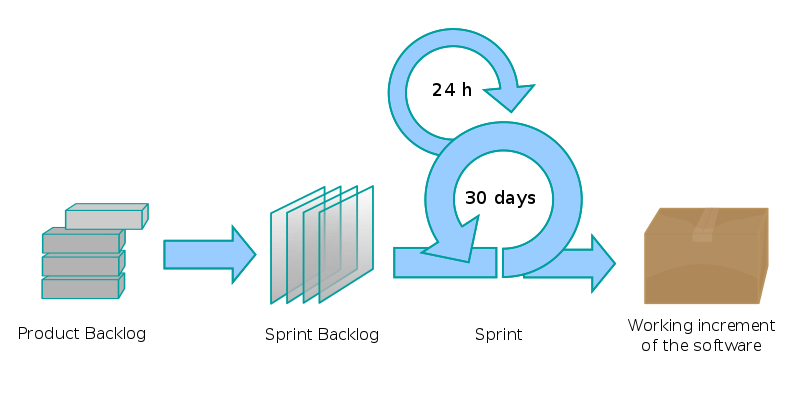
Scrum (software development) Methodology

Scrum is an iterative and incremental agile software development framework for managing software projects and product or application development. Its focus is on "a flexible, holistic product development strategy where a development team works as a unit to reach a common goal" as opposed to a "traditional, sequential approach". Scrum enables the creation of self-organizing teams by encouraging co-location of all team members, and verbal communication between all team members and disciplines in the project.

A key principle of Scrum is its recognition that during a project the customers can change their minds about what they want and need (often called requirements churn), and that unpredicted challenges cannot be easily addressed in a traditional predictive or planned manner. As such, Scrum adopts an empirical approach—accepting that the problem cannot be fully understood or defined, focusing instead on maximizing the team's ability to deliver quickly and respond to emerging requirements.

Roles

There are three core roles and a range of ancillary roles—core roles are often referred to as pigs and ancillary roles as chickens (after the story The Chicken and the Pig).

The core roles are those committed to the project in the Scrum process—they are the ones producing the product (objective of the project). They represent the scrum team.

Product Owner

The Product Owner represents the stakeholders and is the voice of the customer. He or she is accountable for ensuring that the team delivers value to the business. The Product Owner writes (or has the team write) customer-centric items (typically user stories), ranks and prioritizes them, and adds them to the product backlog. Scrum teams should have one Product Owner, and while they may also be a member of the development team, this role should not be combined with that of the Scrum Master. In an enterprise environment, though, the Product Owner is often combined with the role of Project Manager as they have the best visibility regarding the scope of work (products).

Team

The Team is responsible for delivering potentially shippable product increments at the end of each Sprint (the Sprint Goal). A Team is made up of 7 +/- 2 individuals with cross-functional skills who do the actual work (analyse, design, develop, test, technical communication, document, etc.). The Team in Scrum is self-organizing, even though there may be some level of interface with project management offices (PMOs).

Scrum Master

Scrum is facilitated by a Scrum Master, who is accountable for removing impediments to the ability of the team to deliver the sprint goal/deliverables. The Scrum Master is not the team leader, but acts as a buffer between the team and any distracting influences. The Scrum Master ensures that the Scrum process is used as intended. The Scrum Master is the enforcer of the rules of Scrum, often chairs key meetings, and challenges the team to improve. The role has also been referred to as a servant-leader to reinforce these dual perspectives. The Scrum Master differs from a Project Manager in that the latter may have people management responsibilities unrelated to the role of Scrum Master. The Scrum Master role excludes any such additional people responsibilities.

Project Manager

The individual responsible for the success of the project.

The Project Executive and Project Board

Those accountable for the project, particularly where issues and impediments need escalating outside of the Scrum team.

Project Assurance

The individuals with whom the Scrum team will consult in order to achieve their Sprint Goal, and with whom the Product Owner engages to understand what the ranked order of product backlog items should take in order to deliver enterprise value. The Project Assurance group consist of representatives of the Senior Supplier, Senior User and the Project Executive.

Managers

People who control the work environment.

Stakeholders

The individuals, not mentioned above, that often interface both with the Project Assurance group and with the Scrum Team. The stakeholders are sometimes customers, end-users, and vendors. They are people who enable the project and for whom the project produces the agreed-upon benefit[s] that justify its production. They may be involved in the Scrum process during the Sprint Review.

Sprint

A sprint is the basic unit of development in Scrum. The sprint is a "timeboxed" effort, i.e. it is restricted to a specific duration. The duration is fixed in advance for each sprint and is normally between one week and one month.

Each sprint is preceded by a planning meeting, where the tasks for the sprint are identified and an estimated commitment for the sprint goal is made, and followed by a review or retrospective meeting, where the progress is reviewed and lessons for the next sprint are identified.

Meetings

Daily Scrum

Each day during the sprint, a project team communication meeting occurs. This is called a daily scrum, or the daily standup. This meeting has specific guidelines:

• All members of the development team come prepared with the updates for the meeting.
• The meeting starts precisely on time even if some development team members are missing.
• The meeting should happen at the same location and same time every day.
• The meeting length is set (timeboxed) to 15 minutes.
• All are welcome, but normally only the core roles speak.

During the meeting, each team member answers three questions:

• What have you done since yesterday?
• What are you planning to do today?
• Any impediments/stumbling blocks? Any impediment/stumbling block identified in this meeting is documented by the Scrum Master and worked towards resolution outside of this meeting. No detailed discussions shall happen in this meeting.

Backlog refinement (grooming)

This is the process of creating stories, decomposing stories into smaller ones when they are too large, refining the acceptance criteria for individual stories, prioritizing stories on the product backlog and sizing the existing stories in the product backlog using effort/points. During each sprint the team should spend time doing product backlog refinement to keep a pool of stories ready for the next sprint.

• Meetings should not be longer than an hour.
• Meeting does not include breaking stories into tasks.
• The team can decide how many meetings are needed per week.
• Though everything can be done in a single meeting, these are commonly broken into two types of meetings for efficiency:

1. The refinement meeting, when the product owner and stakeholders create and refine stories on the product backlog.
2. The planning poker meeting, when the team sizes the stories on the product backlog to make them ready for the next sprint

Scrum of Scrums

Each day normally after the Daily Scrum:

• These meetings allow clusters of teams to discuss their work, focusing especially on areas of overlap and integration.
• A designated person from each team attends.

The agenda will be the same as the Daily Scrum, plus the following four questions:

• What has your team done since we last met?
• What will your team do before we meet again?
• Is anything slowing your team down or getting in their way?
• Are you about to put something in another team's way?

Sprint planning meeting

At the beginning of the sprint cycle (every 7–30 days), a "Sprint planning meeting" is held:

• Select what work is to be done
• Prepare the Sprint Backlog that details the time it will take to do that work, with the entire team
• Identify and communicate how much of the work is likely to be done during the current sprint
• Eight-hour time limit
• (1st four hours) Entire team: dialog for prioritizing the Product Backlog
• (2nd four hours) Development Team: hashing out a plan for the Sprint, resulting in the Sprint Backlog

End of cycle

At the end of a sprint cycle, two meetings are held: the "Sprint Review Meeting" and the "Sprint Retrospective".

At the Sprint Review Meeting:

• Review the work that was completed and the planned work that was not completed
• Present the completed work to the stakeholders (a.k.a. "the demo")
• Incomplete work cannot be demonstrated
• Four-hour time limit

At the Sprint Retrospective:

• All team members reflect on the past sprint
• Make continuous process improvements
• Two main questions are asked in the sprint retrospective: What went well during the sprint? What didn't went well? What could be improved in the next sprint?
• Three-hour time limit
• This meeting is facilitated by the Scrum Master

Artifacts

Product Backlog

The product backlog is an ordered list of "requirements" that is maintained for a product. It consists of features, bug fixes, non-functional requirements, etc. - whatever needs to be done in order to successfully deliver a working software system. The items are ordered by the Product Owner based on considerations like risk, business value, dependencies, date needed, etc. 
The features added to the backlog are commonly written in story format . The product backlog is the "What" that will be built, sorted in the relative order in which it should be built. It is open and editable by anyone, but the Product Owner is ultimately responsible for ordering the stories on the backlog for the Development Team. The product backlog contains rough estimates of both business value and development effort, these values are often stated in story points using a rounded Fibonacci sequence. Those estimates help the Product Owner to gauge the timeline and may influence ordering of backlog items. For example, if the "add spellcheck" and "add table support" features have the same business value, the one with the smallest development effort will probably have higher priority, because the ROI (Return on Investment) is higher.

The Product Backlog and business value of each listed item is the responsibility of the Product Owner. The estimated effort to complete each backlog item is, however, determined by the Development Team. The team contributes by estimating Items and User-Stories, either in Story-points or in estimated hours

Sprint Backlog

The sprint backlog is the list of work the Development Team must address during the next sprint. The list is derived by selecting stories/features from the top of the product backlog until the Development Team feels it has enough work to fill the sprint. This is done by the Development Team asking "Can we also do this?" and adding stories/features to the sprint backlog. The Development Team should keep in mind the velocity of its previous Sprints (total story points completed from each of the last sprint's stories) when selecting stories/features for the new sprint, and use this number as a guide line of how much "effort" they can complete.

The stories/features are broken down into tasks by the Development Team, which, as a best practice, should normally be between four and sixteen hours of work. With this level of detail the Development Team understands exactly what to do, and potentially, anyone can pick a task from the list. Tasks on the sprint backlog are never assigned; rather, tasks are signed up for by the team members as needed during the daily scrum, according to the set priority and the Development Team member skills. This promotes self-organization of the Development Team, and developer buy-in.

The sprint backlog is the property of the Development Team, and all included estimates are provided by the Development Team. Often an accompanying task board is used to see and change the state of the tasks of the current sprint, like "to do", "in progress" and "done".

Once a Sprint's Product Backlog is committed, no additional functionality can be added to the Sprint except by the team. Once a Sprint has been delivered, the Product Backlog is analyzed and reprioritized, if necessary, and the next set of functionality is selected for the next Sprint.

Increment

The increment is the sum of all the Product Backlog Items completed during a sprint and all previous sprints. At the end of a sprint, the Increment must be done according to the Scrum Team's definition of done. The increment must be in usable condition regardless of whether the Product Owner decides to actually release it.

Burn down

The sprint burn down chart is a publicly displayed chart showing remaining work in the sprint backlog. Updated every day, it gives a simple view of the sprint progress. It also provides quick visualizations for reference. There are also other types of burndown, for example the release burndown chart that shows the amount of work left to complete the target commitment for a Product Release (normally spanning through multiple iterations) and the alternative release burndown chart, which basically does the same, but clearly shows scope changes to Release Content, by resetting the baseline.

FAQ:

Q. How do  you get the user stories which are put in product backlog?

Q. How Scrum master remove impediments to ability of team. If a team member is facing a problem how will he get to know about it and how he fix it. With example?

Q. How project manager is different from Scrum Master and what are it's role and responsibility.

Q. Who verifies the quality of your code. How it is checked for performance?

Q. Explain your daily work routine.

Q. What happen if you are not able to complete your sprint in defined time or week.

Q. According to grooming - "During each sprint the team should spend time doing product backlog refinement to keep a pool of stories ready for the next sprint.". How this is done in daily routine. Who drives it?

Q. In Backlog refinement meeting where "creating stories, decomposing stories into smaller ones when they are too large, refining the acceptance criteria for individual stories, prioritizing stories on the product backlog" is done, who is involved and what role do you play in it?

Q. We have single team or people are divided in multiple teams. If multiple teams then how they communicate with each other.

Q. What you need to do if you are not able to complete a sprint in particular time?

http://en.wikipedia.org/wiki/Scrum_(development)#Product_Backlog

http://en.wikipedia.org/wiki/Agile_software_development

Virtual Columns in Oracle Database 11g Release 1

When queried, virtual columns appear to be normal table columns, but their values are derived rather than being stored on disc. The syntax for defining a virtual column is listed below.

column_name [datatype] [GENERATED ALWAYS] AS (expression) [VIRTUAL]

If the datatype is omitted, it is determined based on the result of the expression. The GENERATED ALWAYS and VIRTUAL keywords are provided for clarity only.

The script below creates and populates an employees table with two levels of commission. It includes two virtual columns to display the commission-based salary. The first uses the most abbreviated syntax while the second uses the most verbose form.

CREATE TABLE employees (
  id          NUMBER,
  first_name  VARCHAR2(10),
  last_name   VARCHAR2(10),
  salary      NUMBER(9,2),
  comm1       NUMBER(3),
  comm2       NUMBER(3),
  salary1     AS (ROUND(salary*(1+comm1/100),2)),
  salary2     NUMBER GENERATED ALWAYS AS (ROUND(salary*(1+comm2/100),2)) VIRTUAL,
  CONSTRAINT employees_pk PRIMARY KEY (id)
);

INSERT INTO employees (id, first_name, last_name, salary, comm1, comm2)
VALUES (1, 'JOHN', 'DOE', 100, 5, 10);

INSERT INTO employees (id, first_name, last_name, salary, comm1, comm2)
VALUES (2, 'JAYNE', 'DOE', 200, 10, 20);
COMMIT;

Querying the table shows the inserted data plus the derived commission-based salaries.

SELECT * FROM employees;

        ID FIRST_NAME LAST_NAME      SALARY      COMM1      COMM2    SALARY1    SALARY2
---------- ---------- ---------- ---------- ---------- ---------- ---------- ----------
         1 JOHN       DOE               100          5         10        105        110
         2 JAYNE      DOE               200         10         20        220        240

2 rows selected.

The expression used to generate the virtual column is listed in the DATA_DEFAULT column of the [DBA|ALL|USER]_TAB_COLUMNS views.

COLUMN data_default FORMAT A50
SELECT column_name, data_default
FROM   user_tab_columns
WHERE  table_name = 'EMPLOYEES';

COLUMN_NAME                    DATA_DEFAULT
------------------------------ --------------------------------------------------
ID
FIRST_NAME
LAST_NAME
SALARY
COMM1
COMM2
SALARY1                        ROUND("SALARY"*(1+"COMM1"/100),2)
SALARY2                        ROUND("SALARY"*(1+"COMM2"/100),2)

8 rows selected.

SQL>

Notes and restrictions on virtual columns include:

• Indexes defined against virtual columns are equivalent to function-based indexes.
• Virtual columns can be referenced in the WHERE clause of updates and deletes, but they cannot be manipulated by DML.
• Tables containing virtual columns can still be eligible for result caching.
• Functions in expressions must be deterministic at the time of table creation, but can subsequently be recompiled and made non-deterministic without invalidating the virtual column. In such cases the following steps must be taken after the function is recompiled:
  • Constraint on the virtual column must be disabled and re-enabled.
  • Indexes on the virtual column must be rebuilt.
  • Materialized views that access the virtual column must be fully refreshed.
  • The result cache must be flushed if cached queries have accessed the virtual column.
  • Table statistics must be regathered.
• Virtual columns are not supported for index-organized, external, object, cluster, or temporary tables.
• The expression used in the virtual column definition has the following restrictions:
  • It cannot refer to another virtual column by name.
  • It can only refer to columns defined in the same table.
  • If it refers to a deterministic user-defined function, it cannot be used as a partitioning key column.
  • The output of the expression must be a scalar value. It cannot return an Oracle supplied datatype, a user-defined type, or LOB or LONG RAW.

Working with Virtual Column:

Creating a Virtual Column:

We will begin by creating a simple table with a single virtual column, as follows.

SQL> CREATE TABLE t
  2  ( n1 INT
  3  , n2 INT
  4  , n3 INT GENERATED ALWAYS AS (n1 + n2) VIRTUAL
  5  );

Table created.

We can see that the virtual column is generated from a simple expression involving the other columns in our table. Note that the VIRTUAL keyword is optional and is included for what Oracle calls "syntactic clarity".

Virtual column values are not stored on disk. They are generated at runtime using their associated expression (in our example, N1 + N2). This has some implications for the way we insert data into tables with virtual columns, as we can see below.

SQL> INSERT INTO t VALUES (10, 20, 30);

INSERT INTO t VALUES (10, 20, 30)
            *
ERROR at line 1:
ORA-54013: INSERT operation disallowed on virtual columns

We cannot explicitly add data to virtual columns, so we will attempt an insert into the physical columns only, as follows.

SQL> INSERT INTO t VALUES (10, 20);

INSERT INTO t VALUES (10, 20)
            *
ERROR at line 1:
ORA-00947: not enough values

Despite the fact that we cannot insert or update virtual columns, they are still considered part of the table's column list. This means, therefore, that we must explicitly reference the physical columns in our insert statements, as follows.

SQL> INSERT INTO t (n1, n2) VALUES (10, 20);

1 row created.

Of course, fully-qualified inserts such as our example above are best practice so this should be a trivial restriction for most developers. Now we have data in our example table, we can query our virtual column, as follows.

SQL> SELECT * FROM t;

        N1         N2         N3
---------- ---------- ----------
        10         20         30

1 row selected.

Our expression is evaluated at runtime and gives the output we see above.

Indexes and Constraints

Virtual columns are valid for indexes and constraints. Indexes on virtual columns are essentially function-based indexes (this is covered in more detail later in this article). The results of the virtual column's expression are stored in the index. In the following example, we will create a primary key constraint on the N3 virtual column.

SQL> CREATE UNIQUE INDEX t_pk ON t(n3);
Index created.

SQL> ALTER TABLE t ADD
  2     CONSTRAINT t_pk
  3     PRIMARY KEY (n3)
  4     USING INDEX;

Table altered.

If we try to insert data that results in a duplicate virtual column value, we should expect a unique constraint violation, as follows.

SQL> INSERT INTO t (n1, n2) VALUES (10, 20);
INSERT INTO t (n1, n2) VALUES (10, 20)
*
ERROR at line 1:
ORA-00001: unique constraint (SCOTT.T_PK) violated

As expected, this generates an ORA-00001 exception.

It follows, therefore, that if we can create a primary key on a virtual column, then we can reference it from a foreign key constraint. In the following example, we will create a child table with a foreign key to the T.N3 virtual column.
SQL> CREATE TABLE t_child
  2  ( n3 INT
  3  , CONSTRAINT tc_fk
  4       FOREIGN KEY  (n3)
  5       REFERENCES  t(n3)
  6  );

Table created.

We will now insert some valid and invalid data, as follows.
SQL> INSERT INTO t_child VALUES (30);

1 row created.

SQL> INSERT INTO t_child VALUES (40);
INSERT INTO t_child VALUES (40)
*
ERROR at line 1:
ORA-02291: integrity constraint (SCOTT.TC_FK) violated - parent key not found

Adding Virtual Column

Virtual columns can be added after table creation with an ALTER TABLE statement. In the following example, we will add a new virtual column to our existing table. We will include a check constraint for demonstration purposes.

SQL> ALTER TABLE t ADD
  2     n4 GENERATED ALWAYS AS (n1 * n2)
  3        CHECK (n4 >= 10);

Table altered.

As stated earlier, an index on a virtual column will store the results of the expression. A check constraint, however, will evaluate the expression at the time of adding or modifying data to the underlying table. This is seemingly obvious, because there is no associated storage structure (i.e. index) with a check constraint.

Our new virtual column, N4, has a check constraint to ensure that the product of the N1 and N2 columns is greater than 10. We will test this, as follows.

SQL> INSERT INTO t (n1, n2) VALUES (1, 2);

INSERT INTO t (n1, n2) VALUES (1, 2)
*
ERROR at line 1:
ORA-02290: check constraint (SCOTT.SYS_C0010001) violated

http://www.oracle-base.com/articles/11g/virtual-columns-11gr1.php

http://www.oracle-developer.net/display.php?id=510

Oracle Database - SQL Plus - Substitution Variables

About
You can define variables, called substitution variables, for repeated use in a single script. Note that you can also define substitution variables to use in titles and to save your keystrokes (by defining a long string as the value for a variable with a short name).

A substitution variable is preceded by one or two ampersands (&).

How to Create a Substitution Variable

Temporary substitution variable:-

When SQL Plus find a substitution variable define by using only one ampersand (&), it tries to replace it with the value of one permanent substitution variable previously defined otherwise, it will prompt you to enter a value that will be use only once.

Permanent Substitution Variables:-

A permanent Substitution Variables is a variable available for the complete session.

Set up a substitution Variable ?

To define a substitution variable, you can use:-

-> DEFINE command

-> Two Ampersands

-> ACCEPT command

-> COLUMN NEW_VALUE

DEFINE command:

         DEFINE L_NAME = SMITH

Note that any substitution variable you define explicitly through DEFINE takes only CHAR values (that is, the value you assign to the variable is always treated as a CHAR datatype). You can define a substitution variable of datatype NUMBER implicitly through the ACCEPT command.

Two ampersands:

SQL*Plus automatically DEFINEs any substitution variable preceded by two ampersands, but does not DEFINE those preceded by only one ampersand.

Oradata@orcl>select &&MySubstitutionVariable FROM dual;

Enter VALUE FOR mysubstitutionvariable: 'Value'

old 1: SELECT &&MySubstitutionVariable FROM dual

NEW 1: SELECT 'Value' FROM dual

'VALUE'

-------

VALUE

Oradata@orcl>DEFINE MySubstitutionVariable

DEFINE MYSUBSTITUTIONVARIABLE = "'Value'" (CHAR)

NOTE: One thing to note here is: Any character string values to be given to variable, must be define in single quotes else the value we provide, will itself be considered as Variable.

Enter value for counter: dsfs

old   5: v_count := &counter;

new   5: v_count := dsfs;

ERROR at line 5:

ORA-06550: line 5, column 12:

PLS-00201: identifier 'DSFS' must be declared

ORA-06550: line 5, column 1:

PL/SQL: Statement ignored

ACCEPT command:
ACCEPT pswd CHAR PROMPT 'Password: ' HIDE 

For a number

ACCEPT salary NUMBER FORMAT '999.99' DEFAULT '000.0' -
PROMPT 'Enter weekly salary: '

PROMPT You have enter: &salary

If we do not Enter salary in defined format, it will keep prompting for right format salary:

SQL> ACCEPT salary NUMBER FORMAT '999.99' DEFAULT '000.0'

4553.223

SP2-0598: "4553.223" does not match input format "999.99"

444.33

COLUMN NEW_VALUE

You can store the value of a column value in a variable using this statement

COLUMN column_name NEW_VALUE variable_name

Example:

define SpoolFileId=idle

column ReleaseId NEW_VALUE SpoolFileId 

select TO_CHAR(SYSDATE,'YYYYMMDD_HH24MMSS_') || '_Release.log' ReleaseId from dual; 

PROMPT The value of SpoolFileId is now: &SpoolFileId

then to define a log file, you can use this statement:

SPOOL '&SpoolFileId'

How to delete a substitution variable?
To delete a substitution variable, use the SQL*Plus command UNDEFINE followed by the variable name.

UNDEFINE MySubstitutionVariable

How to list?

All substitution variables:

To list all substitution variable definitions, enter DEFINE by itself.

SQL> DEFINE

DEFINE _DATE = "14-JUN-10" (CHAR)

DEFINE _CONNECT_IDENTIFIER = "bidb" (CHAR)

DEFINE _USER = "DWH" (CHAR)

DEFINE _PRIVILEGE = "" (CHAR)

DEFINE _SQLPLUS_RELEASE = "1002000300" (CHAR)

DEFINE _EDITOR = "Notepad" (CHAR)

DEFINE _O_VERSION = "Oracle Database 10g Enterprise Edition Release 10.2.0.

4.0 - 64bit Production

With the Partitioning, OLAP, Data Mining and Real Application Testing options" (

CHAR)

DEFINE _O_RELEASE = "1002000400" (CHAR)

DEFINE MY_SUBSTITUTION_VARIABLE = "1" (CHAR)

One substitution variable

PROMPT The value of MySubstitutionVariable is: &MySubstitutionVariable

or

DEFINE MySubstitutionVariable

Parameters:

SET DEFINE:

SET DEFINE defines the substitution character (by default the ampersand ”&”) and turns substitution on and off.

SET DEFINE OFF:

To turn off this functionality (also in SQL Developer).

SET VERIFY:

After you enter a value at the prompt, SQL*Plus lists the line containing the substitution variable twice: once before substituting the value you enter and once after substitution. You can suppress this listing by setting the SET command variable VERIFY to OFF.

SET VERIFY ON. Lists each line of the script before and after substitution. This can be used for debug purpose also. We are able to see which value got assigned to which value variable.

Like in below example:
SQL>  define pswd=12
SQL> define charctr=123
SQL> DECLARE
  2  v_count NUMBER;
  3  v_char VARCHAR2(30);
  4  BEGIN
  5  v_count := &pswd;
  6  v_char := &charctr;
  7  DBMS_OUTPUT.PUT_LINE('First Value of v_count ' ||v_count);
  8  DBMS_OUTPUT.PUT_LINE('Value of v_char ' ||v_char);
  9  END;
 10  /
First Value of v_count 12
Value of v_char 123

PL/SQL procedure successfully completed.

SQL>
SQL> set verify on
SQL> DECLARE
  2  v_count NUMBER;
  3  v_char VARCHAR2(30);
  4  BEGIN
  5  v_count := &pswd;
  6  v_char := &charctr;
  7  DBMS_OUTPUT.PUT_LINE('First Value of v_count ' ||v_count);
  8  DBMS_OUTPUT.PUT_LINE('Value of v_char ' ||v_char);
  9  END;
 10  /
old   5: v_count := &pswd;
new   5: v_count := 12;
old   6: v_char := &charctr;
new   6: v_char := 123;
First Value of v_count 12
Value of v_char 123

PL/SQL procedure successfully completed.

http://www.oracle-base.com/articles/misc/literals-substitution-variables-and-bind-variables.php